figure 1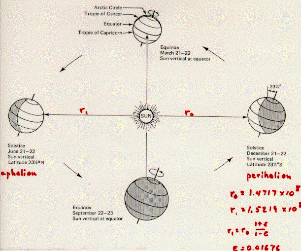 Earth at aphelion and perihelion.
(Lutgens, F.K., and Tarbuck E. J., 1986: The Atmosphere:
An Introduction to Meteorology. Reprinted by permission of
Prentice Hall, Upper Saddle River, N. J., 07458.)
figure 2 Power input from the Sun.
figure 3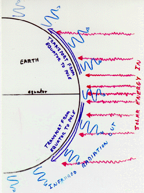 Transport and radiation.
figure 4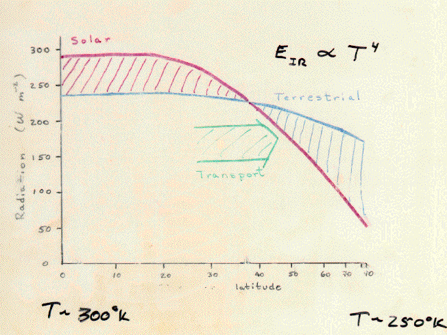 Radiation flux vs. Latitude.
figure 5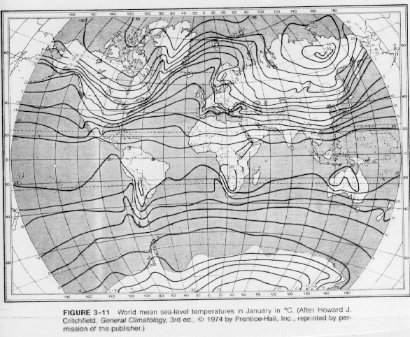 World mean sea-level
temperatures in January.
World mean sea-level
temperatures in January.
(After Howard J. Critchfield, General
Climatology, 3rd ed., 1974 by Prentice-Hall,Inc.)
figure 6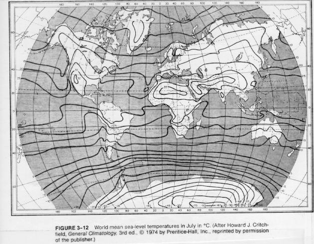 World mean sea-level temperatures in July.
(After Howard J. Critchfield, General
Climatology, 3rd ed., 1974 by Prentice-Hall, Inc.)
figure 7 Structure and temperature of the Atmosphere.
figure 8 Global circulation on a
non-rotating earth.
Global circulation on a
non-rotating earth.
(Lutgens, F.K., and Tarbuck E. J., 1986: The Atmosphere:
An Introduction to Meteorology. Reprinted by permission of
Prentice Hall, Upper Saddle
River, N. J., 07458.)
figure 9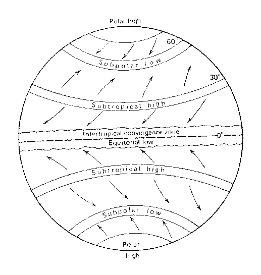 Wind and pressure belts of the earth.
(Lutgens, F.K., and Tarbuck E. J.,
1986: The Atmosphere:
An Introduction to Meteorology. Reprinted by permission of
Prentice Hall, Upper Saddle
River, N. J., 07458.)
figure 10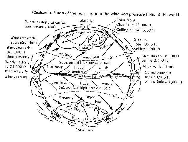 Idealized relation of the polar front to the wind and pressure belts of the
world.
Idealized relation of the polar front to the wind and pressure belts of the
world.
(Donn, W.
L., 1975: Meteorology. McGraw-Hill, Inc., New York, NY. 518
pp.)
figure 11 Idealized diagram showing the relationship between flow near the surface
and aloft.
Idealized diagram showing the relationship between flow near the surface
and aloft.
(Lutgens, F.K., and Tarbuck E. J.,
1986: The Atmosphere:
An Introduction to Meteorology. Reprinted by permission of
Prentice Hall, Upper Saddle
River, N. J., 07458.)
figure 12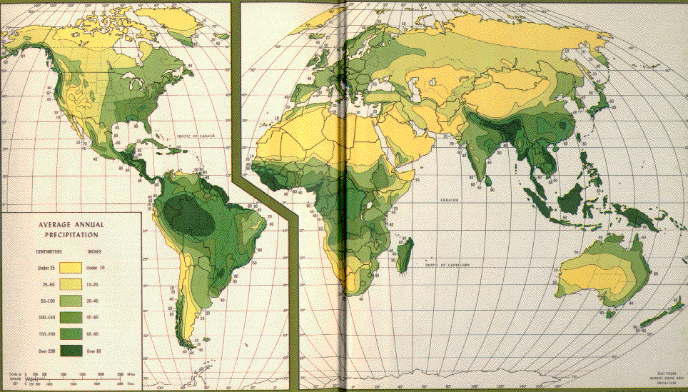 Distribution of average annual precipitation over the continents.
(Trewartha, G. T., 1968: An
Introduction to Climate. McGraw-Hill, Inc. New York, NY, 408 pp.)
figure 13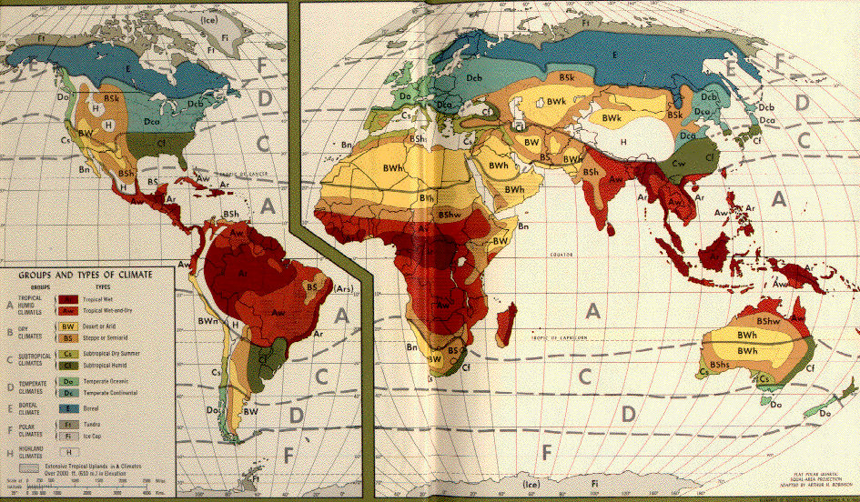 Distribution of types of
climate over the continents. (Trewartha, G. T., 1968: An
Introduction to Climate. McGraw-Hill, Inc. New York, NY, 408 pp.)
Distribution of types of
climate over the continents. (Trewartha, G. T., 1968: An
Introduction to Climate. McGraw-Hill, Inc. New York, NY, 408 pp.)
figure 14 Average annual
precipitation over the tropical Pacific Ocean. (Adapted from R. C.
Taylor, 1973: An Atlas of Pacific Islands Rainfall, Hawaii Institute of
Geophysics.)
Average annual
precipitation over the tropical Pacific Ocean. (Adapted from R. C.
Taylor, 1973: An Atlas of Pacific Islands Rainfall, Hawaii Institute of
Geophysics.)
figure 15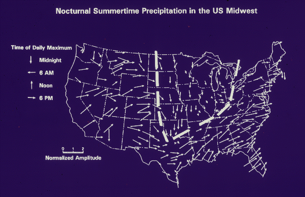 Nocturnal summertime
precipitation in the U.S. Midwest.
Nocturnal summertime
precipitation in the U.S. Midwest.
The earth moves in an elliptical orbit around the sun, being closest to the sun, a distance of 1.47 x 10⁸ kilometers, in December. The distance to the sun is maximum at about 1.52 x 10⁸ kilometers in June. The eccentricity of this elliptical orbit is about 0.016. The time of closest approach is called perihelion (see figure 1) and occurs when the Northern Hemisphere is having its winter, and we call this time the winter solstice. The earth is at aphelion, the furthest distance from the sun, in July when the Southern Hemisphere is having its winter solstice and the Northern Hemisphere has its summer solstice. The midpoints between solstices are called the vernal equinox (equal length of day and night) in spring and autumnal equinox in autumn. The plane of the earth's equator is tipped at an angle of 23.5° to the plane of its orbit around the sun. The earth wobbles slightly so that the tilt actually changes between about 22 and 25 degrees cyclically with a period of about 41,000 years.
The earth/atmosphere/ocean system can be considered as a very large thermodynamic engine that takes energy from the sun, converts it to many other forms, and then releases it back to outer space. The intensity of the sun's radiation reaching the "top" of the atmosphere is 1,380 Wm-2. More power per square meter reaches the earth at low latitudes (closer to the equator) than in the polar latitudes. A simple calculation shows that the power of this engine, shown in figure 2, is about 1.76 x 10¹¹ megawatts. A large power plant in a major city might produce 100 megawatts, so the sun provides the earth with the equivalent of about 2 billion such power plants. Wallace and Hobbs (1977) have calculated magnitudes of natural and anthropogenic heat sources that might alter this engergy balance at the earth's surface.
This energy from the sun is absorbed preferentially in low latitudes in the tropical regions and subtropics (see figure 3). It is transmitted from the tropics toward the polar regions as thermal energy or as latent heat in the form of water vapor. Eventually, this energy is radiated back to outer space in amount equal to the input, giving the earth/atmosphere/ocean system as a whole a thermodynamic balance. The global warming we will discuss later in the course is not a matter of the atmosphere gaining more energy than it is losing, but rather a change in the redistribution of energy in the atmosphere. The earth is not observed to be heating up or cooling down rapidly, and even if we changed the composition of the gases in our atmosphere we don't change this fact that the earth loses the same amount of energy it receives from the sun. When we change the gases in the earth's atmosphere, we change the processes of redistribution: the surface warms, but the stratosphere actually cools.
Energy reaches the surface of the earth in larger amounts in the tropical and subtropical regions (see figure 4). This leads to a net flow of energy in the atmosphere and ocean away from the tropical regions and toward the poles. Ocean water is heated in tropical regions and moves toward the polar regions in currents such as the Gulf Stream off the east coast of the U.S, transporting large amounts of heat from low latitudes to high latitudes. If it weren't for the Gulf Stream, Scandinavia would be about 10°C colder than it is right now. In the atmosphere also, energy moves poleward by means of the global circulation cycle. A subtle way of transforming energy from low latitudes to high latitudes is through latent heat: water that evaporates from the warm tropical oceans is transported as water vapor to higher latitudes. This vapor condenses into liquid and gives up the amount of energy that was used for evaporation in the tropics. Polar regions lose more energy to space than they receive from the sun, so the difference is made up by this transport of energy from low latitudes to high latitudes.
Oceans cover 71% of the earth's surface and land only 29%, with most (90%) of the land being in the Northern Hemisphere. It is notable that in the Southern Hemisphere polar region, the Antarctic continent forms a nearly circular land mass centered on the pole, while in the Northern Hemisphere, the polar region has no comparable land mass.
A graph of average January air temperature near the surface of the earth (see figure 5) shows lines of constant temperature, called isotherms, generally follow the lines of constant latitude running east-west, particularly in the Southern Hemisphere. Over continental areas, these lines are displaced southward in both hemispheres. At this time, the Southern Hemisphere is having its summer, and the land is warmer than the ocean at the same latitude because the land absorbs more energy than the water. This agrees with our experience that you can cool off during a warm summer day by going to the ocean. In the Northern Hemisphere, of course, January corresponds to winter, and the southward displacement of the isotherms means that the land is colder than the water at the same latitude.
Average July temperatures (see figure 6) show isotherms being displace northward in both hemispheres in response to the land being warmer than the water at the same latitude in the Northern Hemisphere and cooler than the water in the Southern Hemisphere.
The vertical distribution of global average temperature, as seen in figure 7, shows that the surface of the earth has a temperature of about 288 Kelvin or about 59°F. The temperature decreases with height from the surface to about 10 kilometers, equivalent to an altitude of about 6 miles. This level is called the tropopause which marks the upper boundary of the troposphere. Above this level, in what is known as the stratosphere, the temperature remains constant with height at a value of about -55°C to a height of about 20 km, above which it increases to a maximum at the stratopause, an altitude of about 50 km. This plot is a very idealized picture of the atmospheric temperature profile. Over the polar regions the tropopause will be only perhaps 8 km and over the tropics it may reach 17 km. It also is interesting to note that the coldest tropopause temperature is over the tropics where it might typically reach -80°C.
This temperature structure is very critical for how moisture and trace gases move in the atmosphere. Air in the troposphere is quite well mixed. Moisture, pollutants, or trace gases that are put into the atmosphere at the surface are usually mixed quite thoroughly throughout the troposphere within a matter of 2 or 3 days. And precipitation processes usually wash soluble particles out of the troposphere in 1 to 3 weeks. If foreign material gets into the stratosphere, however, it may persist there for 1 to 3 years. So, for instance, the soot from the Kuwaiti oil fires during the Gulf War was confined to the troposphere and was washed out before it traveled very far from the fire region, whereas dust from the eruption of Mount Pinatubo in the Philippines in 1991 spewed large amounts of dust into the stratosphere that reduced sunlight levels over the globe for about 3 years. The fact that the stratosphere is a very stable region that doesn't foster mixing will be important later when we discuss ozone.
We have seen that the tropical regions receive more energy per unit time than the polar regions and that this energy is redistributed around the planet by the movement of the atmosphere and ocean. To understand how this happens, we need to review the effect of the earth's rotation on air and ocean movement. If we forgot for a moment that the earth rotates on its axis, like figure 8, then the excessenergy in tropical areas would cause the warm, less dense air to rise. As it moves away from the earth's surface, it would be replaced by air coming from either of the poles. Over North America, a persistent wind from the north at the surface would carry air to the tropics where it would rise and drift northward at high levels to the North Pole where it would sink to the surface and then return to the south. A symmetrically similar pattern would develop in the Southern Hemisphere.
In reality, however, since we observe motions relative to fixed locations on the earth, the rotation of the earth creates an "apparent" force on any moving object or fluid. We call this the Coriolis force. In the Northern Hemisphere it exerts a force to the right (and to the left in the Southern Hemisphere) so a parcel of air moving toward the North Pole will be deflected toward the right. Air moving toward the equator is deflected to the right in the Northern Hemisphere and to the left in the Southern Hemisphere, resulting in a persistent surface wind from the northeast on the north side of the Equator and from the southeast on the south side of the Equator. This creates what we call a sub-tropical high-pressure region at about 30° north and south of the Equator where air moving poleward at high levels does not go directly to the polar region but, rather, is deflected eastward and subsides back to the earth's surface (see figure 9).
On the poleward side of this circulation cell in each hemisphere is another cell that rotates in the opposite direction: air at the surface moves toward the pole, and air at high levels moves toward the tropics. This leads to a generally westerly wind in the middle latitudes (30° to 60°) north and south of the Equator). In the United States, we have a generally west-to-east movement of weather systems. At latitudes higher than 60o, a third circulation cell exists with surface flow away from the pole and poleward flow aloft. The Coriolis force creates winds generally from the east at the surface at these high latitudes.
If you recall looking at the animation of the cloud motions (1.0 MB) from the Internet exercises, you should have observed motions of the clouds in the tropical regions to be from east to west, while those in middle latitudes were from west to east. Because the preceding description of the global circulation is somewhat idealized, there may be occasional exceptions to this simplified picture of atmospheric motions.
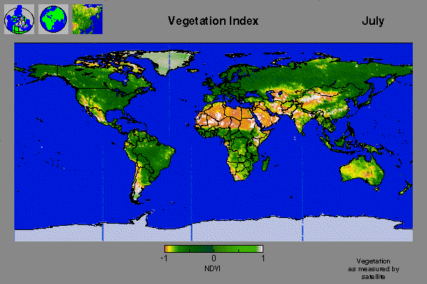
Rising air in the tropical regions may reach altitudes of 10 km or more. As this air rises, it cools, and the further it rises the more it cools. In fact the coldest temperatures in the lower atmosphere are not over the polar regions but over the tropics near the base of the stratosphere. Intense precipitation resulting from this rising air has eliminated most of the moisture, so this air moving toward the poles is very dry. As this air sinks in the high pressure belts at 30° north and south, it is compressed and warms, just as air in a bicycle pump is warmed by compression. This warm, dry air produces a cloud free environment with sunny dry, even desert, climates at these latitudes. A quick look at the vegetation maps (July, 1995) for the planet shows the paucity of vegetation at these latitudes.
The weather and climate at midlatitudes is dominated by the motion of the westerly wind belts in the North and Southern Hemisphere, as shown in figure 10. This region is the battleground between cold air masses originating in polar regions and warm air masses arising from the tropics. The boundary between these two air masses at the earth's surface defines the position and character of the weather fronts (cold fronts, warm fronts, stationary fronts). At the tropopause, this boundary marks the position of the jet stream, a high-speed current of air moving generally parallel to the air-mass boundary from west to east. Cold, dense polar air occasionally sloshes toward the Equator, dragging with it the frontal boundary (cold front) at the surface and the jet stream aloft.
The jet stream is linked to surface weather patterns through horizontal convergence and divergence patterns. A sketch of the jet stream shows that the streamlines come together in some regions leading to higher speed flow. These regions are linked to downward moving air at midlevels and high-pressure zones at the surface where air is turned by the Coriolis force to form a clockwise rotation. On the other hand, regions of divergence aloft tend to draw air upward from the surface forming low-pressure centers at the surface, as can be seen in figure 11. If this rising air is warm and moist, it produces cloudiness and precipitation normally associated with low-pressure centers. Forecasting the weather is then an attempt to forecast how these low-pressure centers develop and move. Because surface weather features are very strongly linked to the upper level flow, the first computer forecast models developed by applied mathematicians and meteorologists were designed to predict the characteristics and movement of the "middle" of atmosphere, at 500 millibars or 5-6 km above the surface. Patterns and movement of this region give strong clues about weather at the surface.
The persistent flow across warm ocean surfaces into the tropical regions moves significant amounts of moisture into regions of convergence and upward motion. A map of global rainfall shows tropical areas receive very large amounts of precipitation along what is called the Intertropical Convergence Zone (ITCZ), shown in figure 12. Some regions receive in excess of 5 meters of rain annually. We will revisit the details of tropical precipitation when we discuss the El Nino.
The atmospheric circulation also controls the precipitation patterns in the subtropical high-pressure belts near 30° north and south of the Equator. And the movement and development of low-pressure zones along the frontal boundaries in the middle latitudes likewise govern precipitation in these regions. Comparison of global maps of precipitation and vegetation reveals the importance of precipitation amounts in determining the level of biological production, as is shown in figure 13. Even from this general viewpoint, we can see that changes in the global circulation patterns and precipitation patterns can have significant impacts on global vegetation (see figure 14). We will consider these issues again when we examine the carbon cycle of the planet and the land-use practices now in place over large regions of the earth's surface.
Regional precipitation patterns may be governed by peculiar processes not linked to the global circulation. In the Midwest US, for instance, the summertime precipitation pattern is quite different from the rest of the US, as can be seen from the map showing the timing of summertime rainfall. Most regions of the US have precipitation occurring during the middle to late afternoon, in response to warming of the surface and evaporation of moisture that leads to cloud development and precipitation. The Midwest, by contrast, has a maximum rainfall occurring at night, as is illustrated in figure 15. The Great Flood that occurred during the summer of 1993 produced much of its heaviest rainfall after sunset. The reason for this is that the Midwest experiences what are called mesoscale convective complexes (MCC). These large-scale systems originate in the Great Plains to the west in the afternoon and drift into the Midwest after sunset. Instead of dissipating after the loss of solar heating at sundown, these MCCs draw additional moisture from the low-level jet stream from the south that serves as an efficient conveyor belt of moisture from the Gulf of Mexico. The intensification of the jet after sunset fuels the afternoon thunderstorms from the plains region and allows them to persist and grow as they move across the Midwest after sunset.
These regional precipitation processes are not completely understood, and how they will be affected by changes in the global climate due to greenhouse warming is not very well known. Estimations of how precipitation patterns change under global warming are among the largest uncertainties of our projections of climate change. And because of the strong link between global precipitation patterns and vegetation, projections of impacts on agriculture and natural systems also have large uncertainty.