
|
|
|
|
|
|
|
|
|
|
|
|
|
|
|
|||||||
|
|
|
|
|
|
|
|
|
||
1-14: Global Warming Potential | 1-14: En Espa�ol | 1-14: Em Portuguêus |
Introduction
We have discussed how the impact of increased greenhouse gas
concentrations relates to increased radiative forcing, or heating, of the
atmosphere. To calculate the magnitude of future global warming due to
increasing greenhouse-gas concentrations, we need two items: (1)
projections of future atmospheric concentrations of greenhouse gases and
(2) a global climate model to translate increased radiative forcing into
changes in surface temperatures. In this unit, we focus on the
projections of future concentrations of greenhouse gases. The topic of
global climate models will be covered in the second block of this course.
Global Warming Potential (GWP)
Figure 1 sketches the impact over time of
adding one unit of a greenhouse gas to the atmosphere.
Lifetime of the gas is the primary factor in determining the overall warming effect of the gas. Carbon dioxide, for instance, which has an atmospheric lifetime of about 120 years, continues to contribute to radiative forcing, although with decreasing impact, for many decades. And other species, like some CFCs that have very long lifetimes, may contribute to global warming for many centuries.
We define the "global warming potential" (GWP) as the total impact over time of adding a unit of a greenhouse gas to the atmosphere. It is calculated by multiplying the effect of the instantaneous radiative forcing by the concentration of gas added and integrating over time from 0 to some arbitrary time period, T. Carbon dioxide, for instance, has relatively low radiative forcing but a very high volume of gas annually added to the atmosphere and a long atmospheric lifetime, so it has a very high GWP. The CFCs on the other hand have low concentrations but very high radiative forcing factors and very large lifetimes, so they also have very high GWPs.
Atmospheric Lifetime and GWP Compared to CO2
Figure 2, from the IPCC report, gives
the atmospheric
lifetime and GWP compared to carbon dioxide for various gases over several
different time horizons.
From this table you can see that methane, a short-lived species, contributes 62 times as much as carbon dioxide to the Global Warming potential over twenty years, but over longer periods of time its impact decreases because of its shorter lifetime (relative to carbon dioxide). Contrast this with CFC-13, which has a lifetime of 400 years: its GWP increases as the time horizon of consideration increases. This points out the importance of knowing the lifetime of these chemicals that we put into the atmosphere.
A byproduct of increased methane in the stratosphere is an increase in stratospheric water vapor, which arises due to oxidation of methane. So even after stratospheric methane is destroyed, its contribution to global warming continues through the presence of water vapor.
Global Warming Contribution
Figure 3 gives the relative contribution to global warming
caused by different chemical species, with an assumed 100-year time horizon
and 1990 emissions estimates.
Carbon dioxide, with its enormous annual increase in concentration, contributes most, at 61%. Methane is second in importance, at 15%, CFC-12 is third, contributing 7%, and nitrous oxide fourth with 4% of the warming under these assumptions. If we took the 500-year horizon, the percentages would change, with longer-lived species contributing larger percentages.
The question now is how do we estimate future emissions of greenhouse gases? Past trends can be used as a starting point, but future emissions will be determined by a complex combination of economic, regulatory, and societal factors. Some, like the CFCs, can be changed relatively quickly by switching to different chemicals for certain industrial and manufacturing processes and consumer products (e.g., eliminating Styrofoam cups that use CFCs). Others like the burning of fossil fuels cannot be changed very quickly, even if society chooses to do so (it takes many years to put a nuclear power plant in operation to replace a coal-fired plant). Since no one can predict the future with any certainty, we resort to considering several different scenarios, each of which gives a specific set of assumptions on economic, political, and social factors.
Different Future Socio-Economic Development Paths
Assumptions of future economic conditions have two dimensions:
Figure
4 shows four families of scenarios depending on these behavioral
patterns of future societies as described in the Special Report
on Emissions Scenarios (SRES). Each of these four families has a "storyline" that
describes the global population and energy consumption patterns and the associated
greenhouse gas emissions:
Scenario A1 represents high economic
growth and global perspectives to economic and environmental issues. It is further subdivided into
a scenario continuing to emphasize intensive use of fossil fuels (A1FI), one being energy intensive but with emphasis on use of
non-fossil energy (A1T), and a scenario with a balance of fuel sources between fossil and non-fossil (A1B). Global population peaks
about 2050 and then declines.
Scenario A2 assumes self-reliance and
preservation of local identities. Developing regions are less influenced by developed countries,
so that, for instance, fertility follows local historical traditions rather than patterns of developing countries. Global population
does not peak in mid-century. Economic development is linked to regional rather than global patterns.
Scenario B1 has global population
peaking around 2050 and declining thereafter. Economic growth is more globally linked but with
introduction of clean and resource-efficient technologies. Social equity is emphasized with global attention to economic, social and
environmental problems. However, there are no global restrictions on emissions of greenhouse gases.
Scenario B2 has an increasing global
population, but somewhat less than
A2, which does not peak in mid-century. Emphasis is on a local
approaches to addressing economic, social, and environmental sustainability. Emphasis is on environmental protection and social equity
through local approaches. Economic development is not as rapid as in B1
and A1 but with more diverse technological change.
Resulting Emissions Scenarios and Atmospheric Greenhouse Gas
Concentrations
Each of these scenarios creates a somewhat different pattern of greenhouse
gas emissions. The following figures show the emissions corresponding to
each of these scenarios and the time record of atmospheric concentrations of
greenhouse gases that will result from each scenario.
* Adapted from IPCC, 2001: Climate Change
2001:
Synthesis Report. A contribution of Working Groups I, II, and III to the
Third Assessment Report of the Intergovernmental Panel on Climate
Change [Watson, R.T. and the Core Writing Team (eds.)]. Cambridge
University Press, Cambridge, United Kingdom, and New York, NY, USA, 398
pp.
N2O
Emissions
and Concentration*
CH4
Emissions and Concentration*
SO4
Emissions and Concentration*
Global Cooling
The emphasis to this point has been on atmospheric constituents that lead to global warming. However, other factors lead to a cooling, as described in Figure 6. Atmospheric factors shown in this sketch include natural factors such as upper sides of clouds, volcanic eruptions, natural biomass burning, and dust from storms. In addition, human-induced factors such as biomass burning (forest and agricultural fires) and sulfate aerosols from burning coal contribute tiny particles that contribute to cooling.
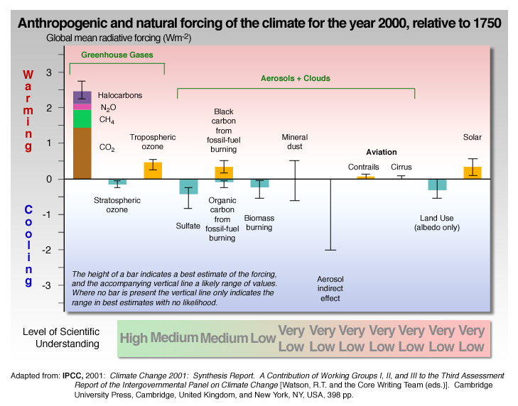
Combined Effects on Radiative Forcing
Best estimates of the combined warming and cooling
effects, as reported in the 2001 report of the Intergovernmental Panel on
Climate Change, are shown in
Figure 7.
Also included in this graph is the effect of changing land use on surface
albedo (absorption of solar radiation at the surface). To underscore the
importance of human-induced activities, the right-hand-most bar in the
graph shows the contribution to radiative forcing from variations in
output of the sun. These results show that current anthropogenic
greenhouse gas forcing is about 5 times larger than natural variation for
2000, and, from the results of Figure 6, could be 10 to 20 times larger
than natural variation by the end of the 21st century. Plots of current
and future projected concentrations of carbon dioxide with past values
over geological time scales are given in Figures 8-11. Noteworthy are
both the magnitudes of the future projections and the timescales over
which these changes are occurring, compared to natural variations.
The future emission scenario that ultimately occurs
will determine how the long term trend of atmospheric CO2
changes. Figure 8 shows
current levels
compared to the historical record of the past 400,000 years. Figure 9 gives the likely
CO2
level in 2040 since we have little hope for abrupt reductions from current
emissions patterns. An upper limit target that frequently is quoted is to
stabilize (not exceed) twice the pre-industrial value (see Figure 10). If we follow
the
"business as
usual" A1T scenario, the atmospheric CO2 level in 2100 is shown
in Figure 11.
In Block 2 of this course we will examine, by use of
global climate
models, the impact on climate due to these changes in atmospheric
constituents.
Return to Unit
Page