
|
|
|
|
|
|
|
|
|
|
|
|
|
|
|
|||||||
|
|
|
|
|
|
|
|
|
||
Carbon Content of Ecosystems on Land
Figure 1 gives estimates of the carbon content of several
different major ecosystems on land. For each, the estimated
land area is in
hectares (1 hectare is 10,000 square meters or 2.47 acres) and carbon content in
units of 1015 grams ( =1 petagram or 1 gigaton). From
this table we can see that
tropical seasonal forests and tropical evergreen forests account for nearly half of
the plant carbon on the planet. The tropical rain forests, of course, have
received considerable attention in the scientific literature and in the public press
as being particularly valuable because they contain so much of the earth's plant
carbon and also because they serve as hosts for perhaps even millions of
biological species, many of which have not yet even been
cataloged.
Boreal forests (high latitudes, mostly Canadian, Scandanavian, and Russia) have carbon approximately comparable with the tropical evergreen forests, and temperate forests add somewhat smaller but significant amounts. Grasslands and pasture in temperate zones, such as native prairie in the US Midwest, contribute a relatively small amount to the vegetation carbon total compared to the forested regions of the tropics or boreal areas. It is informative, however, to consider the amount of plant carbon per unit area in each land class (divide the values in the second column by the values in the first column to get values in the fourth column). Cultivated land in temperate zones supports only slightly less than half as much carbon per hectare as native temperate prairies. By breaking the prairie sod, the early settlers in the Midwest began the process of reducing plant carbon in the region by over 40%. This is, of course, in addition to the accompanying deforestation that took place at the prairie margins. It might be tempting to argue that a lush Iowa cornfield with 30,000 or more plants per acre would have more plant carbon than native prairie vegetation, but the data suggest otherwise.
Carbon Content in Soils
The next column lists carbon in soils. Boreal forests and tundra and
alpine meadow contribute almost identical amounts to the planetary total soil
carbon. Temperate grasslands and pasture contribute nearly as much
total soil carbon as the boreal forest soils, but somewhat less on a per-hectare
basis. The per-hectare values of the fourth and fifth columns can be expressed
in kilograms per square meter by dividing these numbers by 10. Hence,
tropical evergreen forests have about 17.7 kilograms per square meter of carbon
in the vegetation, while the temperate grassland and pastures have about
0.7 kilogram per square meter. The most notable entry in this column is
the enormous carbon density in soils of swamps and marshes, being over 2
1/2 times as much as the next largest entry.
Tillage of soil increases microbe activity in the soil and leads to rapid conversion of soil carbon to CO2. The small marshes and wetlands (known as prairie potholes) that once covered the Iowa, Dakota, and southern Canada landscape, were rich in soil carbon as suggested by the carbon table. Draining and cultivating these regions has resulted in the loss of significant amounts of soil carbon. One of the benefits of modern minimum-tillage and no-tillage practices is that they increase amounts of carbon that are stored in the soil.
Changes in Carbon Content
Figure 2 shows changes in carbon reserves for each land-use
category between 1850 and 1980. In this table, positive numbers indicate a
decrease in the carbon content in that particular land use category. Note that
some areas show an increase in total carbon because the area of this category
has increased and not because the carbon per unit area has increased. For
example, cultivated lands in temperate zones have doubled their carbon content
between 1850 and 1980, but this is due to a doubling of the area in this land
classification. The amount of carbon per unit area in this land-use type has
been essentially constant.
Agricultural and forestry management practices can have a significant effect on the earth's global carbon cycle. Soil tillage practices, crop choices, and plantation and forestry management practices all impact the global carbon cycle. High latitude continental areas have vast boreal forests and frozen tundra that store carbon for longer periods of time. Many biological and physical processes depend on temperature: higher temperatures tend to accelerate these processes. For example, cooking food speeds up the physical transformation processes. In tropical areas where the temperature is high but moisture is not limiting, growth and decay processes occur very rapidly, whereas at high latitudes and high altitudes (mountainous areas) they proceed very slowly. Disturbances to plant ecosystems that occur in areas of where transformations proceed slowly take much longer to recover than in warmer climates.
Agricultural soils have lost about a third to one half of their native carbon. Agriculture, by use of alternative tillage practices and also by eliminating excessive use of nitrogen fertilizers, may help to reduce atmospheric carbon dioxide by allowing more carbon to be stored in the soil. Nitrogen fertilizers stimulate soil processes and accelerate the transformation of soil carbon to carbon dioxide: reducing excessive use of nitrogen fertilizer reduces the amount of soil carbon lost to the atmosphere.
Carbon Dioxide
Carbon dioxide is a friendly gas: at atmospheric concentrations, even
double the present amount, it is not harmful to humans, since it is odorless,
colorless, and does not react in the human body. And plants grow more
vigorously in enriched CO2 environments, so why do we raise the concern
about its increase? A significant characteristic of carbon dioxide is that it has a
very long effective lifetime in the atmosphere. Figure
3 shows
atmospheric concentration excess as a function of time. This graph provides an
answer to the following question: If we put one extra kilogram of carbon
dioxide into the atmosphere, how quickly will the atmospheric CO2 level return to
its original level? This curve shows that 60 years have elapsed before
half of the initial kilogram is removed and about 200 years elapsed before
two-thirds of the initial
amount it lost. The lifetime of carbon dioxide in the
atmosphere is obviously very long. This means that large amounts of carbon
dioxide presently being put into the atmosphere by burning fossil fuels and
deforestation will, on average, be around for many decades.
Figure 4 gives the global distribution of carbon as best known in 2001.
Atmospheric Carbon Dioxide Inputs
We have identified numerous natural processes that put significant
amounts of carbon dioxide into the atmosphere, much larger amounts than are
contributed by burning fossil fuels or deforestation. And the uncertainty in the
magnitudes of these natural sources is large, perhaps much larger than the
amounts of anthropogenic (human) sources. It is then tempting to attribute
the increase to some error in our estimate of natural sources and not blame
humans.
Figure 5 shows convincing evidence that the source of much of the increase in carbon in the atmosphere is fossil fuels. Carbon has three isotopes, C12, C13, and C14. Carbon 12 is the most abundant, and C13 and C14 are produced from C12 in the biosphere by cosmic radiation. Once produced, the C13 or C14 will slowly decay back to C12. Fossil fuels represent carbon that has been removed from the biosphere for centuries and buried under the surface of the earth where it is shielded from cosmic radiation. The C13 and C14 of such carbon stores have had a long time to decay back to C12 without production of new amounts of C13 and C14. Therefore, fossil fuels are almost pure C12. Combustion of fossil fuels then adds C12 to the atmosphere but not C13 or C14. This means that the relative amount of C13 and C14 should decrease as the level of C12 is increased. The accompanying graph shows measurements of the partial fraction of C14 in the atmosphere over the last 130 years. The data clearly show a decrease in the relative abundance of C14 during the last few decades. These data provide strong evidence implicating fossil fuels as a major contributor to the increase in atmospheric carbon dioxide. The data for C13 provide additional confirming evidence.
The fate of carbon dioxide put into the atmosphere by burning fossil fuels can be summarized as shown in Figure 6 which shows the number of petagrams of carbon per year taken up by the ocean and atmosphere and ocean together between 1800 and 1990. The difference in these two curves, labeled as the "residual", is the estimated amount that must be accounted for by changes in vegetation uptake and changes in land use (e.g., deforestation, carbon or carbon-sequestering capability lost due to urbanization). The figure on the right gives the best estimate of the amount due to land use. The remainder, labeled "missing sink", suggests that there is some unaccounted-for loss of carbon from the atmosphere/ocean system. Speculation is that the boreal forest or high-latitude oceans may be responsible, but more data are needed to confirm the identity of the missing sink. A recent paper suggests this missing sink is over the central part of the US.
Future Anthropogenic Emissions of CO2
We've looked at atmospheric carbon dioxide from the past up to the
present, and now it might be informative for us to look to the future.
Anthropogenic emissions of carbon dioxide to the atmosphere in the future,
which occur mainly due to burning of fossil fuels, are very closely tied to
economic development. Strong economic activity in developed countries and
modernization of developing countries both relate closely to the production of
electrical energy, use of fossil-fuel burning machines, and the use of cement.
These agents of growth all produce carbon dioxide as byproducts. Presently the
anthropogenic production of carbon dioxide increases about 2% per year. We
can use different economic growth rates to project future anthropogenic
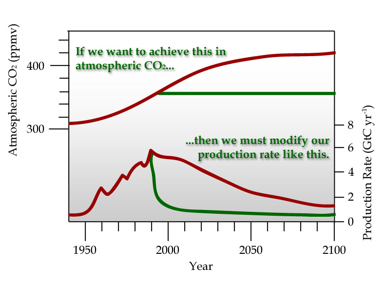
production of carbon dioxide, as is shown in Figure 7a. Here it can be seen
that by continuing on our present rate of growth, atmospheric carbon dioxide
levels will reach 600 ppm by about 2050. Reducing our growth in production
to zero (keeping emissions constant at current levels) reduces the level to 440
ppm by 2050. If our goal were to limit atmospheric levels to less than 400
ppm, we would have to reduce emissions by 2% per year. If we turned off all
fossil-fuel burning power plants, stopped using automobiles, and eliminated all
other anthropogenic emissions, the atmospheric carbon dioxide concentration
would return to about the 1980 level by 2050 (Figure 7b).
This figure reveals the dilemma that we face if we seek to limit the growth of atmospheric carbon dioxide. We seem destined to have a very high level of carbon dioxide in the earth's atmosphere, compared with levels of the last 160,000 years, by the middle of the next century.
Let's briefly summarize what we have learned about the carbon cycle to this point. During the period of 1860-1994 there has been about 241 gigatons of carbon emitted to the atmosphere by fossil fuel combustion, and the rate in 1990 was 6.0 gigatons of carbon into the atmosphere due to deforestation, and the present rate is about 1.6 gigatons per year. Apparently deforestation is on the increase again in South America because of the renewed demand for farm land. Atmospheric carbon dioxide concentrations have increased from about 275 ppm in the middle of the last century to the present value of about 370 ppm in 2001. We understand the basic features of the carbon cycle quite well. It is possible to construct quantitative models to use as a guide in projecting the CO2 concentrations. The uncertainties of the projections of likely future CO2 changes on the basis of a given emission scenario are considerably less than those of the emission scenarios themselves. We cannot project our economic growth very well, but if we could, we probably could project our CO2 levels quite accurately. It will require some reduction in emissions growth rate to keep from doubling our atmospheric carbon dioxide level over the next 50 years.
Emission Statistics
In 1998, greenhouse gas (GHG) emissions in the US were nearly 10% higher
than 1990 levels, and could rise 47% above 1990 levels by 2020,
according to two new reports from the US Department of Energy's
Energy Information Administration (EIA) . GHG emissions in 1998 totaled 1,803
million metric tons of carbon equivalent (MtCe), with CO2 representing
about 83% of the total, according to Emissions of Greenhouse Gases in
the United States 1998. Emissions rose only slightly (0.2%) from 1997 to
1998, the lowest annual growth rate since 1991, when emissions actually
fell slightly owing to economic recession.
Warmer winter weather (13% warmer than in 1997) reduced consumption of winter heating fuels; however, this was offset by warmer summer weather (14% warmer than average and 22% warmer than in 1997) that led to greater use of air- conditioning and thus higher electrical production. Low oil prices also led to "large-scale" fuel switching from natural gas to oil for electrical generation -- increasing oil consumption in this sector by 42%. Transportation emissions grew by 2.4% from 1997 to 1998, primarily owing to an increase in gasoline consumption. Overall, CO2 emissions climbed 0.3% from 1997 to 1998, and are now 11% higher than 1990 levels.
Meanwhile, methane emissions dropped 1.4% between 1997 and 1998, and are now nearly 5% lower than in 1990. EIA attributes the decline to increased capture of methane from landfills, mandated by EPA regulations but spurred on by operators trying to meet a deadline to receive tax credits for landfill gas recovery projects. Emissions of HFCs, perfluorocarbons, and sulfur hexafluoride -- accounting for just over 2% of total GHG emissions on a carbon equivalent basis -- grew by 5% between 1997 and 1998, and are now some 82% higher than in 1990.
Finally, EIA estimates that forest regrowth in the US currently sequesters some 209 MtC annually -- about 14% of US CO2 emissions. However, the report notes that this rate of sequestration is slowing as these regenerating forests reach maturity.
Despite the low emissions growth rate from 1997 to 1998, EIA does not expect this trend to continue, according to the reference case forecasts in its Annual Energy Outlook 2000. This analysis projects that carbon emissions from energy use will increase an average of 1.3% annually, growing to 33% above 1990 levels in 2010 and 47% above 1990 levels in 2020. The forecast for 2020 is slightly higher than projected in last year's Outlook, owing to higher projected economic growth, travel, and electricity generation.
Methane
Methane is
another atmospheric constituent whose concentration has
increased in recent years. Methane is also a greenhouse gas that is about
twenty times as effective on a molecule for molecule basis as is CO2. One
methane molecule will absorb 20 times as much infrared radiation as CO2. Its
lifetime is much shorter than carbon dioxide, however, so this partially
compensates for its higher absorption.
Actually, methane is the most rapidly increasing greenhouse gas. Figure 8 shows the recent concentration of methane, in parts per million by volume (ppm), to be about 1.7 ppm. Updated values are given by the Carbon Dioxide Information Analysis Center. Sometimes methane concentration is given in parts per billion by volume (ppb), and then would have a value of 1700 ppb. The numerical values show that methane is much less abundant than carbon dioxide which has a present concentration of about 360 ppm. However, the curve shows that the concentration increased by more than 1% per year from 1978 - 1987. If we look at a longer term, as shown in figure 8, we see that concentrations have increased substantially since the Industrial Revolution. Estimate of atmospheric methane from a thousand years ago suggest values around 0.7 ppm (700 ppb) which were constant until about the late 1700s. Since that time, concentrations have more than doubled. If we examine the Antarctic ice core data going back 160,000 years, we see that methane levels fluctuated between about 300 parts per billion and 700 parts per billion until the Industrial Revolution when it began its climb to near 1700 parts per billion (Figure 9).
Sources of Methane
What are the sources of methane (Figure 10)? The 1992
Report of the Intergorvernmental Panel on Climate Change (IPCC) lists the largest
natural source of methane to be wetlands, which produce 115 teragrams (1012
grams) of carbon annually. The uncertainty in these numbers, however, is very
large. Termites are very significant producers of methane in that they eat wood
and release methane in the digestion process. The ocean produces about 10
teragrams per year of methane, and fresh water and methane hydrate contribute
smaller amounts.
Anthropogenic sources include the coal mining, natural gas, and petroleum industries at about 100 teragrams, which is almost as much as natural wetlands. Rice paddies produce on the order of 60 teragrams by means of a process where methane produced in the soil is able to travel up to the hollow stem of the rice plant and be released into the atmosphere without passing through the water, which would tend to suppress the evolution of methane gas (Figure 11).
Enteric fermentation, the digestion process in ruminant animals such as cattle, sheep and goats, produces very large amounts of methane. Animal wastes produce about 25 teragrams; domestic sewage, 25 teragrams; landfills about 30 teragrams; and biomass burning, about 40 teragrams. Some landfills are now being tapped for their methane as a source of power production. This makes good sense on the basis of global warming in addition to getting a "free" source of combustion gas. Burning one methane molecule produces one CO2 molecule, but the global warming potential is reduced by a factor of 20 because the carbon dioxide molecule is only about one-twentieth as effective as the methane molecule in absorbing infrared radiation.
Increases in animal populations are contributing to the increase in atmospheric methane. Figure 12 shows recent increases in several different classes of livestock. If humans continue to have an appetite for meat, the upward trend in animal production and resulting production of methane will likely continue. A particular situation to watch is the development and possible dietary changes in China. If we examine the eating habits of Japan, South Korea, and other Asian nations that have developed very rapidly, one of the significant changes that occurs during economic development is that people's eating habits change from eating primarily grains, mainly rice in these cases, to substantial increases in meat. The big question on the horizon right now is what's going to happen in China? China has an enormous population and it is developing extremely rapidly. If China follows the pattern of other Asian nations, the demand for meat will increase dramatically. I have estimated that if every person in China at a MacDonald's Quarter Pounder every 10 days, raising the beef to meet this demand would consume all the corn grown in Iowa.
Sinks for Methane
Sinks for methane include atmospheric removal of about 470 units,
removal by soil of about 30 teragrams, leaving an atmospheric increase of about
32 units. By taking subtotals of natural and anthropogenic sources, it is easy
to see that humans contribute at least as much as natural sources and possible
much more. Such numbers as these are consistent with the observed build-up
of methane in the atmosphere in the last 200 years. (See
Figure 10.)
Methane Concentrations Leveling Off
Between 1978 and 1987 atmospheric methane levels increased by more than 1% per
year (Figure 8).
After 1987 methane continued to increase, but at a slower rate. Now, recent
measurements report that the data for year 1998 through 2005 show a rather
abrupt hault to the rise in this powerful greenhouse gas. Reasons for this
change may be repairs to leaky oil and gas lines and storage facilities and
reduced emissions from rice paddies, coal mining and natural gas production.
These results suggest that the human intervention may play a strong role in
reducing further increase in this greenhouse gas.
Carbon Monoxide
Carbon monoxide is another carbonaceous gas in the earth's atmosphere
that participates in the global carbon cycle. Figure 13 gives the
sources and sinks of carbon monoxide in teragrams of carbon per year. Fossil
fuel combustion is a significant source, as is biomass burning. Carbon
monoxide also can be produced in secondary oxidation reactions with methane
or non-methane hydrocarbons (NMHC). Major sinks include reaction with
the hydroxyl radical and soil uptake. These estimates also carry large
uncertainties, but again it is very likely that anthropogenic sources dominate
natural sources. Carbon monoxide is much more reactive than carbon dioxide,
so its lifetime in the atmosphere is comparably shorter.
Measurements of N2O from satellites are described by
NASA.
Conclusions
Updated atmospheric CO2 graphs can be obtained here